
Transformers
Published:
Transformers: This post contains my notes throughout years on different transformers. These notes are very crude and not edited yet (more like my cheat sheets), but I thought to share it anyway. Please let me know if you have any comments or if you find any mistakes. Images used in this blogpost, otherwise mentioned, are all taken from the papers on each model.
Table of Contents
Attention is all you need
Paper from Google
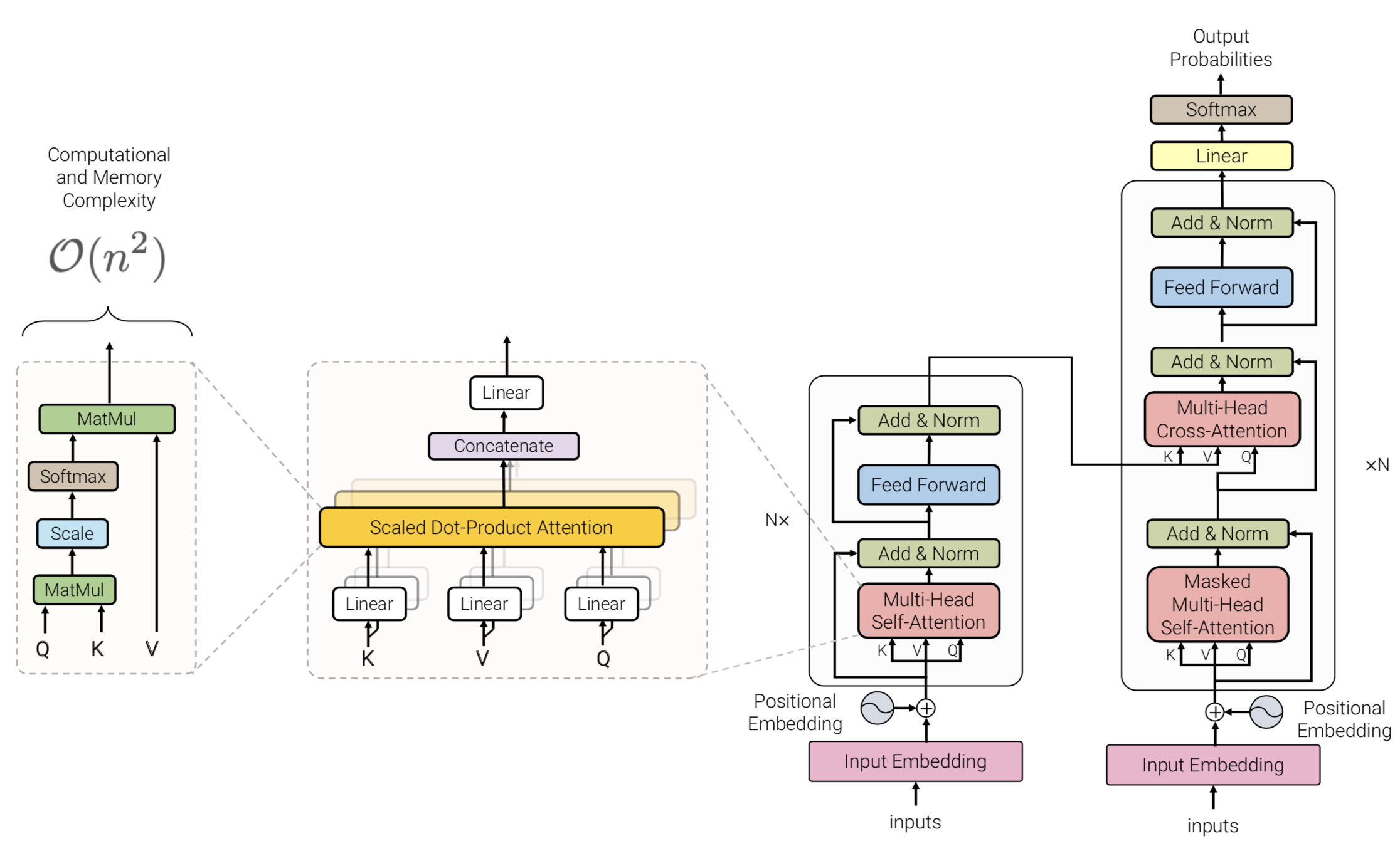
The transformer era began with this paper from Google. The architecture consists of an encoder and a decoder block to solve machine translation.
Positional encoding Using sin and cos functions, the earlier dimensions have smaller wavelengths and can capture short-range offset, while the later dimensions can capture longer distance offset. This blog does a great job in explaining the positional encoding.
Transformer blocks are characterized by a multi-head self-attention mechanism, a position-wise feed-forward network, layer normalization modules, and residual connectors. The input to the Transformer model is often a tensor of shape RB × RN , where B is the batch size, N the sequence length.
There are residual self-attention blocks which are efficient in transferring positional encodings to the top layers. For a deeper understanding of transformers, I recommend reading the original paper, this blogpost by from Rémi Louf and The Annotated Transformer by Alexander Rush After “Attention all you need” BERT from Google and GPT from OpenAI were introduced which I will exlained leter in this post.
BERT
BERT: Pre-training of Deep Bidirectional Transformers for Language Understanding
Paper from Google
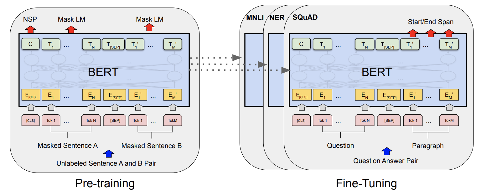
BERT is based on subword token encoding and multi-layer transformer architecture. The transformer blocks are the same as the original transformer blocks introduced in “Attention is all you need” paper, however BERT only uses the Encoder part of the transformer architecture (and this is why it is not suitable for text generation tasks).
BERT uses a huge corpus of data for pre-training the model on a self-supervised task, masked language modeling. They mask tokens in the text and the decoder should predict the masked tokens. BERT masks 15% of the tokens. From the 15% selected tokens, 80% of them are actually being masked, 10% replaced by a random token, and 10% unchanged and the model is expected to predict all of these tokens (and the loss of all predictions will be backpropagated). See my colab notebook for the code of masking.
You may ask why not masked all the 15% of tokens?! The reason is if you are masking all the tokens masked, the model will try to only represent the masked tokens and ignore the rest. When you replace tokens by random or leave them unchanged, the model needs to make a prediction for every single token, because it doesn’t have a clue which ones are replaced by a random token which one is original, so it will make an effort to predict all the tokens and learn from all of them. After pretraining, the model can be fine-tuned on many language understanding tasks such as translation, NER, QA, and text classifications.
One of the disadvantages of BERT is that BERT fails to model the joint probability of the predicted tokens, i.e. it assumes that predicted tokens ([MASK]s) are independent.
GPT
Improving Language Understanding by Generative Pre-Training
Paper from OpenAI 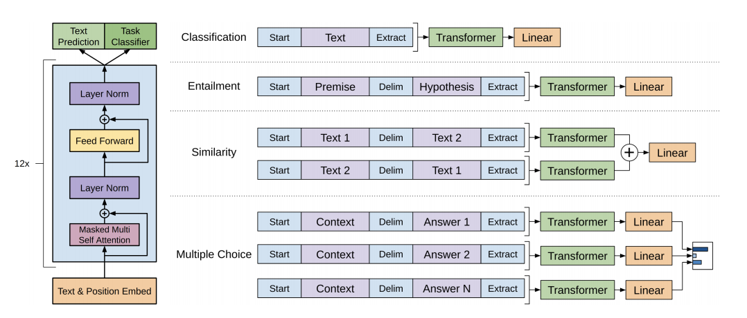
ALL GPTs have only the transformer decoder (and not the encore part). In GPT first the model is pre-trained for LM tasks (causal LM) and then fine-tuned on the final task. They found that including language modeling as an auxiliary objective to the fine-tuning helped learning by (a) improving generalization of the supervised model, and (b) accelerating convergence. So the final objective is L3(C) = L2(C) + λ ∗ L1(C) in which L2 is the objective for labeled data and L1 is the objective for LM. Overall, larger datasets benefit from the auxiliary objective ( λ ∗ L1(C) ) but smaller datasets do not.
For Training, they used a modified version of L2 regularization with w=0.01 on all non-bias or gain weights. For the activation function, they used GELU. They also learned the position embeddings instead of the sinusoidal version. For fine-tuning, 3 epochs were sufficient for the most task and they set λ =0.5
GPT1 was trained on book corpus (about 7K unpublished books), the context size (number of tokens) was 512.
GPT2 was trained on outbound links from Reddit (the articles which were linked from Reddit) which received at least 3 karma (keeping only posts with a high number of upvotes) resulted in 45M links after filtering (removing Wikipedia pages etc) and they ended up with 8M webpages, 40GB of text (around 10B tokens). GPT2 model has 1.5B parameters (when 48 layers), size of vocab is 50.257K, context size is 1024 tokens (remember BERT was 512), and batch size 512. GPT2 achieves SOTA in 7 out of 7 NLP benchmarks.
Differences between GPT and GPT2: Layer normalization was moved to the input of each sub-block, similar to a residual unit of type “building block” (differently from the original type “bottleneck”, it has batch normalization applied before weight layers). An additional layer normalization was added after the final self-attention block. A modified initialization was constructed as a function of the model depth. The weights of residual layers were initially scaled by a factor of 1/√n where n is the number of residual layers. Use a larger vocabulary size and context size.
GPT2 vs GPT3 Data compression
GPT2 data compression: (tokens/parameters) = 10B/1.5B=6.66 This means in GPT2 there is one parameter for every 6.66 tokens.
GPT3 has 175B parameters and is trained on 499B tokens (from common crawl, webtext2, books1, books2, Wikipedia). The 175 Billion parameters need 175*4=700GB memory (floating-point needs 4 bytes)
GPT3 data compression (tokens/parameters) = 499/175=2.85 GPT3 has lower data compression compared to GPT2 so, with this amount of parameters, whether the model functions by memorizing the data in the training and pattern matching in inference.
GPT-3 shows that it is possible to improve the performance of a model by “simply” increasing the model size, and in consequence, the dataset size and the computation (TFLOP) the model consumes. However, as the performance increases, the model size has to increase more rapidly. Precisely, the model size varies as some power of the improvement of model performance. Remember language model performance scales as a power-law of model size, dataset size, and the amount of computation.
XLNet
Generalized Autoregressive Pretraining for Language Understanding” from Carnegie Mellon and Google Research.
Paper from
Similar to Bert, XLNet is using booksCorpus and English Wikipedia (13GB of plain text). In addition, authors include Giga5(16 GB) ClueWeb (19G after filtering), Common Crawl (110 GB after filtering) for pretraining. In total, they have 32.89 B tokens.
XLNet-Large is similar to BERT-Large in model size and they use a sequence of 512 tokens. The authors observe with a batch size of 8192, it took 5.5 days to train, and still, it underfits the data. XLNet achieves SOTA on 18 out of 20 NLP tasks.
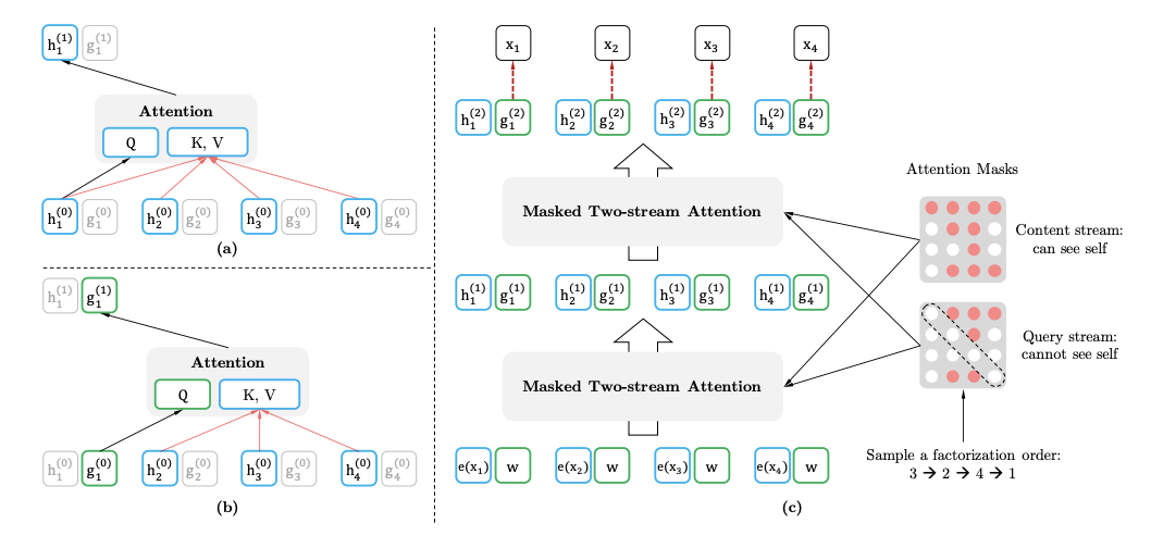
XLNet combines the bidirectional capability of BERT with the autoregressive technology of Transformer-XL. Remember the disadvantage of BERT is that BERT fails to model the joint probability of the predicted tokens, i.e. it assumes that predicted tokens ([MASK]s) are independent, AR models eliminate the independence assumption made in BERT (the shortcoming of BERT are resolved in T5 as well with a less complicated approached compared to XLNet).
XlNet has advantages of both AR (auro-regressive) and AE (auto-encoding) models. Since an AR language model is only trained to encode a unidirectional context (either forward or backward), it is not effective at modeling deep bidirectional contexts. On the contrary, downstream language understanding tasks often require bidirectional context information. This results in a gap between AR language modeling and effective pretraining. Firstly, instead of using a fixed forward or backward factorization order as in conventional AR models, XLNet maximizes the expected log likelihood of a sequence w.r.t. all possible permutations of the factorization order. Thanks to the permutation operation, the context for each position can consist of tokens from both left and right. In expectation, each position learns to utilize contextual information from all positions, i.e., capturing bidirectional context.
XLnet uses the following techniques:
- relative positional embeddings (instead of absolute position for each token)
- extending attention queries across previous (not trainable) token sequences
- using permutations to consider masked language modeling to looks ahead to future tokens Implementing the aforementioned techniques is complicated and perhaps this is why I haven’t seen XLNet being widely used.
RoBERTa
RoBERTa: A Robustly Optimized BERT Pretraining Approach
Paper from UW and Facebook AI
In the RoBERTa paper, the authors first performed an ablation study on the effect of different BERT’s parts of performance on end tasks. They observed that larger batch size increases the performance, the NSP doesn’t affect performance (sometimes no NSP increases performance) and tries static vs dynamic masking and observed dynamic masking improved performance. They gathered all the learning and proposed RoBERTa (Robustly optimized BERT approach) Specifically, RoBERTa is trained with dynamic masking, FULL-SENTENCES without NSP loss, large mini-batches, and a larger byte-level BPE.
So in short, RoBERTa provides a better pre-trained compared to BERT by
- training the model longer, with bigger batches, over more data; - removing the next sentence prediction objective;
- training on longer sequences; and
- dynamically changing the masking pattern applied to the training data.
They realized BERT is greatly under fitted, so they used 160GB of text instead of the 16GB dataset originally used to train BERT, batch size of 8K instead of 256 in the original BERT base model. They also removed the next sequence prediction objective from the training procedure as they realized it does not help the model. RoBERTa matches XLNet models on the GLUE benchmark and sets a new state of the art in 4/9 individual tasks of GLUE. Also, they match SOTA on SQuAD and RACE.
ALBERT
ALBERT: A Lite BERT for Self-supervised Learning of Language Representations
Paper from Google Research and Toyota Technological Institute
ALBERT incorporates two-parameter reduction techniques that lift the major obstacles in scaling pre-trained models.
- Factorized embedding parameterization The first one is a factorized embedding parameterization. In BERT, XLNet, and RoBERTa the WordPiece embedding size E is tied with the hidden layer size H, i.e., E ≡ H. By decomposing the large vocabulary embedding matrix into two small matrices, they separate the size of the hidden layers from the size of vocabulary embedding. This separation makes it easier to grow the hidden size without significantly increasing the parameter size of the vocabulary embeddings. Instead of projecting the one-hot vectors directly into the hidden space of size H, they first project them into a lower dimensional embedding space of size E, and then project it to the hidden space. By using this decomposition, they reduce the embedding parameters from O(V × H) to O(V × E + E × H). This parameter reduction is significant when H ≫ E Cross-layer parameter sharing.
- The second technique is cross-layer parameter sharing. This technique prevents the parameter from growing with the depth of the network. Both techniques significantly reduce the number of parameters for BERT without seriously hurting performance, thus improving parameter-efficiency. An ALBERT configuration similar to BERT-large has 18x fewer parameters and can be trained about 1.7x faster. The parameter reduction techniques also act as a form of regularization that stabilizes the training and helps with generalization.
Inter-sentence coherence loss
To further improve the performance of ALBERT, they also introduce a self-supervised loss for sentence-order prediction (SOP). This forces the model to learn finer-grained distinctions about discourse-level coherence properties. SOP is a much more difficult task compared to NSP and SOP can solve the NSP task to a reasonable degree. Remember in NSP two sentences/segments are different in terms of topic and are not coherent. However, in SOP only the order of sentences is swapped, hence the topic is still the same but are not coherent hence the task is harder (remember topic prediction is easier to learn compared to coherence prediction and topic prediction overlaps with what is learned using the MLM loss)
ALBERT doesn’t use dropout. ALBERT v2 — This throws a light on the fact that a lot of assumptions are taken for granted are not necessarily true. The regularisation effect of parameter sharing in ALBERT is so strong that dropouts are not needed. (ALBERT v1 had dropouts
BART
Denoising Sequence-to-Sequence Pre-training for Natural Language Generation, Translation, and Comprehension
Paper from Facebook AI 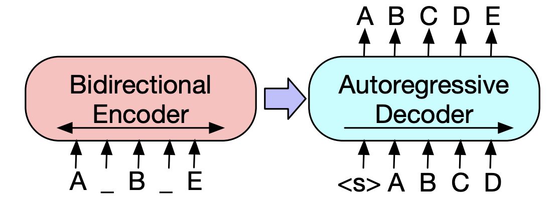
a denoising autoencoder for pretraining sequence-to-sequence models. BART is trained by (1) corrupting text with an arbitrary noising function, and (2) learning a model to reconstruct the original text. It uses a standard Transformer-based neural machine translation architecture.
They evaluate a number of noising approaches, finding the best performance by both randomly shuffling the order of the original sentences and using a novel in-filling scheme, where arbitrary length spans of text. BART is particularly effective when fine-tuned for text generation but also works well for comprehension tasks.
BART contains roughly 10% more parameters than the equivalently sized BERT model.
Pretraining: Token Masking like BERT Token Deletion Random tokens are deleted from the input. The model must decide which positions are missing inputs. Text Infilling A number of text spans are sampled. Each span is replaced with a single [MASK] token.
Sentence Permutation A document is divided into sentences based on full stops, and these sentences are shuffled in random order. Document Rotation A token is chosen uniformly at random, and the document is rotated so that it begins with that token.
AMBERT: A Multigrained BERT
Paper by ByteDance
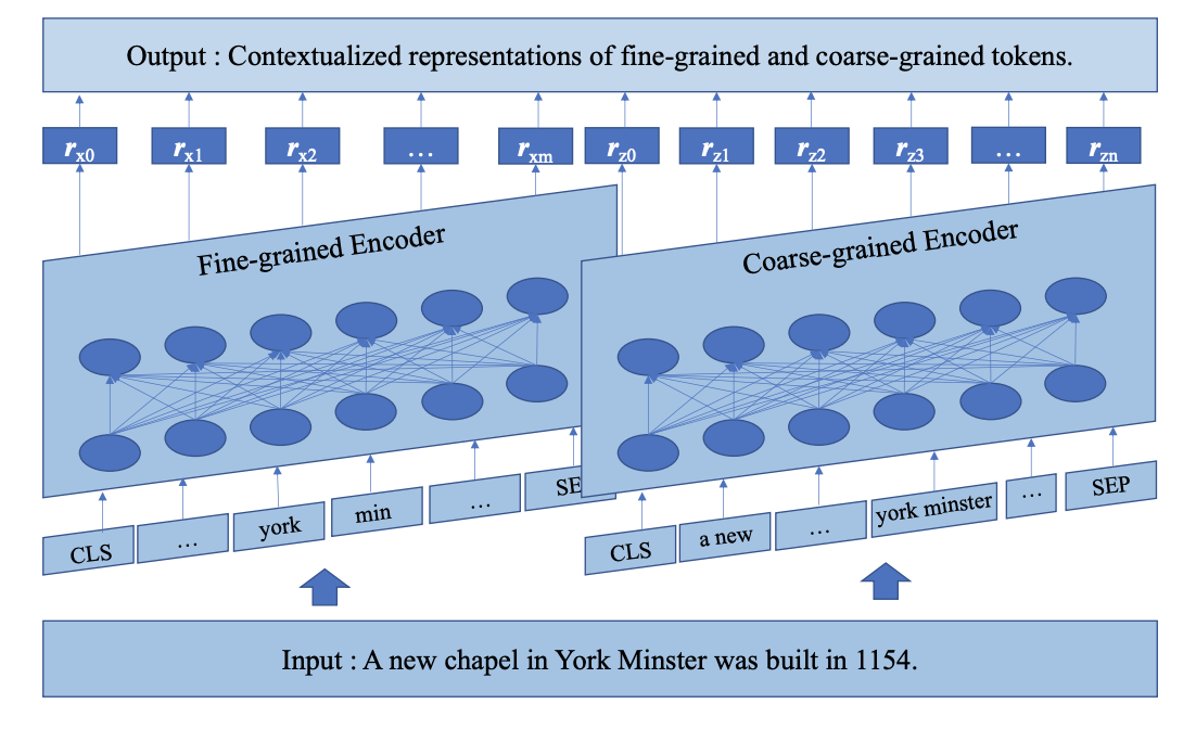
AMBERT proposes a simple twist to BERT: tokenize the input twice, once with a fine-grained tokenizer (subword or word level), and once with a coarse-grained tokenizer (phrase level).
The two inputs share a BERT encoder. A forward pass through the model consists of the following two steps: text tokens → token embeddings (via separate weights): Each list of tokens (one fine-grained, one coarse-grained) is looked up in its own embedding matrix and turned into a list of real-valued vectors. token embeddings → contextual embeddings (via shared weights): The two real-valued vectors are fed into the same BERT encoder (a stack of Transformer layers) — which can be done either sequentially through a single encoder copy, or in parallel through two encoder copies with tied parameters. This results in two lists of per-token contextual embeddings. Because AMBERT uses two embedding matrices (one for each tokenization), its parameter count is notably higher than BERT’s (194M vs 110M for the English Base models). However, latency remains relatively unchanged since AMBERT solely adds a new set of dictionary lookups